
Singapore Polytechnic - Data analytics with Knime
Link to github: Github link
KNIME KNIME is a free and open-source data analytics, reporting and integration platform that integrates various components for machine learning and data mining through its modular data pipelining “Lego of Analytics” concept . A graphical user interface and use of JDBC allows assembly of nodes combining different data sources, including preprocessing (ETL: Extraction, Transformation, Loading), for modeling, data analysis and visualization without, or with only minimal, programming. www.knime.com/about
Introduction
Statistics and Analytics for Engineers(SAE) is module that introduces student to statistic and data analytics concepts to solve problems encountered through the course of their studies. One of the ways that this is achieved is through the project detailed in this post.
This project was originally split into 2 milestones spread out over about 11 weeks. I have combine both milestones into a single post.
All data used is dummy data provided by Singapore Polytechnic(SP) for educational purposes
The team
My team consisted of the following people, all of us were from Singapore Polytechnic(SP) taking Diploma in Electrical and Electronic Engineering(DEEE)(As of 29 August 2021)
- Khiu Kim Hong
- Ngo Bing Han
- Bryan Ng Xu hen
Problem statement
Student performance monitoring has been one of the crucial KPI in educational institutions. If these institutions are able to foresee any students more likely to be at-risk (do badly in exams), lecturers can do an intervention program prior to the exams. There are several attributes being collected and decided to do something useful with these data.
Your task is to develop a predictive model on who is likely to be at-risk (do badly in exams) and requires extra support. This model should provide an indication if similar pattern was seen for future students; the model should flag out the record and intervention program should be undertaken.
The report
Note The report that the team wrote is uploaded verbatim. This will allow readers to compare and contrast the quality of work against future post.
1. Business understanding
Context “Target score” refers to the final score a student obtain at the final stage of the whole course.
The educational institution wants to be able to predict which students are most likely to be ‘at-risk’ and require assistance. The attribute that the team will focus on is ‘Target score’. The rationale behind the choice is 2-fold. Firstly, the team believes that ‘Target score’ is a good indication of a student’s performance as it is the aggregate of all a student’s subject scores. Secondly, as ‘Target score’ is recorded at the year of the school year, the team believes that enough time has passed for students to acclimatize to the educational institution and hence a student’s performance should not be heavily affected by transitory issues.
2. Data understanding and preparation
The following table illustrates how the data was cleaned and the rationale behind each step along with the respective nodes used in knime.
 |
| Knime workflow for overall data cleaning, including split for students not taking science |
| Step number | Nodes used | Rationale |
|---|---|---|
| 1 | File Reader | Imported CSV into KNIME for analytics |
| 1A | Statistics | To obtain a general overview of data and determine which attribute has missing values. |
| 2 | String Manipulation | ‘Gender’ is standardised to ‘M’ and ‘F’ from ‘Male’, ‘Female’, ‘M’ and ’F’. |
| 3 | Columns Rename | ‘Entrance test’, ‘Eng point’, ‘Math point’ and ‘CCA point’ are renamed to ‘Entrance Test Score’, ‘Entrance Eng Score’, ‘Entrance Math Score’ and ‘Entrance CCA point’ respectively to make their affiliation to the entrance test clearer. All attributes with ‘Att’ are standardised to ‘att’. All ‘?’ are removed. ‘Programming subject score’ is changed from integer to double data type for standardisation purposes. |
| 4 | Rule Engine | 1 instance of “Not reported” Annual household income level was replaced with “High”. The team believes that this was caused by human error and replaces the unknown value with the mode of the category. |
| 5 | Column Filter | ‘Min. subject score’ is dropped due to redundancy with ‘Overall first sem. score’. “Student ID” is dropped as it is deemed irrelevant. |
| 6 | Missing Value | The following attributes with missing categorical data need to be filled with their respective modes: ‘Internet’, ‘Romance’. The team set the missing value threshold at 5%, as both values are above 5% neither are filtered. |
| 7A | Row Filter, Reference Row filter |
82 students who did not take science subjects are filtered and examined separately. The information of these 82 students were filtered into their own separate branch (See 7B). |
| 7B | Row Filter, Reference Row filter, Column filter |
As these students do not take science, both science related columns are dropped entirely. |
| 8 | Rule Engine, Missing Value, Reference Row filter | The 21 rows in ‘Science Subject Attendance’ with a value of 0 are replaced with the median value of ‘Science Subject Attendance’. The value of zero is likely human error and hence should be rectified. Median is selected as the spread of values are heavily positively skewed. |
| 9 | Colour Manger | Used to set colours to make the graph easier to read |
| 10 | String Manipulation | Added ‘Disc’ to Discipline, ’Int’ to Internet, ‘RO’ to Romance, ‘PT’ to ‘Part-time, ‘InC’ to ‘Income’ and ‘CON’ to ‘Conduct’ responses to better fit the sunburst chart. Separate nodes are needed as different columns are being appended. |
3.Data exploration
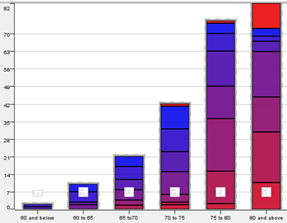
Of the 314 students whose data we analysed, 82 of them did not take science as a subject, hence these records of these students are filtered and analysed separately. The students taking science will henceforth be referred to as Group 1 and those not taking science be referred to as Group 2. The team created a histogram of the ‘Target score’ using a numeric binner. ‘Target score’ was binned into increments of 5 for ranges: 60 to 80. Bins for ‘60 and below’ and ‘80 and above’ was also created
 |
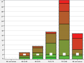 |
| Histogram for group 1 | Histogram for group 2 |
The histogram of both groups are negatively skewed, indicating that students generally did well for their first semester with the majority getting between 75 to 85 marks. The histograms also show us roughly how many students are performing poorly and resources can be provisioned accordingly.
The team hypothesized that the following factors have an impact on student performance and investigated accordingly.
- Entrance scores have an impact on performance
- Students’ attendance has an impact on performance
- Extraneous factors have an impact on student performance
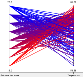
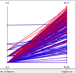
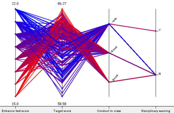
Entrance scores have an impact on performance.
Using parallel plots, the team outlined the entrance scores to the ‘Target score’ of both groups of students. It is important to note that lower entrance score equates to better performance, while higher ‘Target score’ indicates better performance.
 |
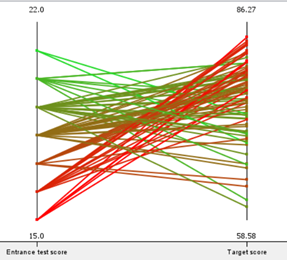 |
| Parallel coordinate of Group-1 | Parallel coordinate of Group-2 |
As seen from the parallel coordinates of both groups, in general students with good entrance scores will continue to do well, and vice versa, barring outliers. Therefore, the team concludes that entrance score is a factor that determines a students’ 1st semester score.
Attendance has an impact on performance. Secondly, using parallel coordinates, the team charted the overall attendance to the ‘Target score’ of both groups of students.
 |
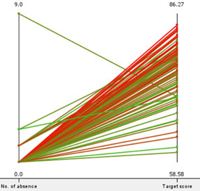 |
| Parallel coordinate of Group-1 | Parallel coordinate of Group-2 |
As shown by both graphs, students of both groups with a small range of attendance yielded a large range of grades. This implies that attendance does not have a strong correlation with performance. As such, we can conclude that attendance does not have a strong impact on performance.
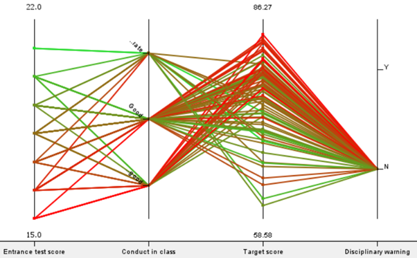
Extraneous factors have an impact on performance.
Lastly, using a sunburst and conditional box plot, the team investigated if extraneous factors have any effects on student performance. The team defines extraneous factors as circumstances not directly related to academics. As such, the following attributes are considered extraneous factors: ‘Annual Household Income level’, ‘Part Time Job?’, ‘Internet?’, ‘Conduct in class’, ‘Disciplinary warning’, ‘Romance?’.
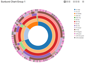 |
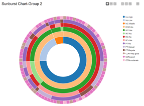 |
| Sunburst chart of Group-1 | Sunburst chart of Group-2 |
The sunburst chart is intended to give a quick overview of the demographics of Group 1 and Group 2.
For both groups, most of the students are from a high-income household, do not have a discipline record, have internet access, are not involved in a romantic relationship, do not have a part time job and have either ‘good’ or ‘very good conduct’.
Next, we will analyse each of the extraneous factors one by one to see if it affects student performance and see if it relates to the sunburst chart.
 |
 |
| Boxplot of ‘Annual Household Income level’ to performance of Group-1 | Boxplot of ‘Annual Household Income level’ to performance of Group-2 |
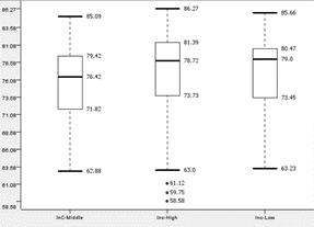
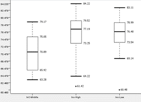
Students with an annual household income of ‘High’, ‘Middle’, ‘Low’ will be referred to as ‘InC-High’, ‘InC-Middle’ and ‘InC-Low’ respectively.
For Group-1, all 3 boxplots show relatively similar medians, Quarter 1, Quarter 3 and Interquartile range. InC-Middle has the widest range and the lowest lower fence.
For Group-2, the sample size of InC-Middle is too small to perform meaningful analysis. InC-High and InC-Middle shows similar performance due to similar medians, Quarter 1, Quarter 3, and upper and lower fences.
Thus, we can conclude that annual household income is not a factor that affects the student’s performance.
 |
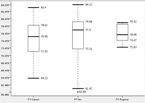 |
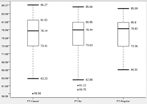
| Boxplot of ‘Part time job?’ to performance of Group-1 | Boxplot of ‘Part time job?’ to performance of Group-2 |
According to the boxplot, the median for both groups are similar, ranging from 75.55 to 78.44. All 6 graphs show similar interquartile ranges between 4 to 7. Barring outliers, Group-1 shows an overall range of about 19 to 23 and Group-2 shows an overall range of about 5 to 7. Thus, we conclude that having part-time jobs does not have a strong impact on student performance.
 |
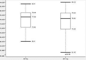 |
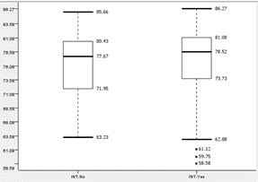
| Boxplot of ‘Internet?’ to performance of Group-1 | Boxplot of ‘Internet?’ to performance of Group-2 |
Students with internet access and without internet access will be referred to as ‘INT-Yes’ and ‘INT-No’ respectively. All 4 graphs show similar medians and interquartile ranges. Although INT-No of Group-1 has a slightly lower upper and lower fence than INT-Yes, while INT-No of Group-2 has a marginally higher lower fence than INT-Yes. As such, the team concludes that internet access is not a large factor for student performance.
The team also notes that INT-Yes of both groups contain outliers that perform worse than the lower fence of INT-No. This is the opposite of the team’s expectation that students without internet would perform worse than those with internet.
 |
 |
| Boxplot of ‘Conduct in class’ to performance of Group-1 | Boxplot of ‘Conduct in class’ to performance of Group-2 |
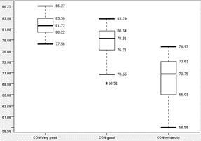
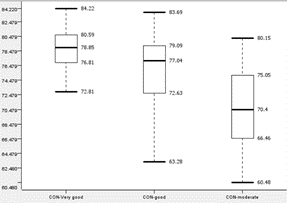
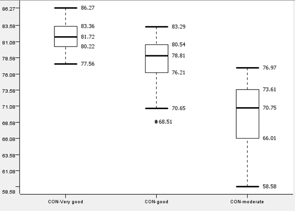
Students with conduct of ‘Very Good’, ‘Good’, ‘Moderate’ will be referred to as ‘CON-Very Good’, ‘CON-Good’ and ‘CON-Moderate’ respectively.
All graphs across both groups display similar trends. CON-Moderate has a lower median, Quarter 1, Quarter 3 and upper and lower fences than the other 2 graphs. It also has a higher interquartile range, despite having similar overall ranges compared to the other graphs. It is also noted that the upper fence of CON-Moderate is close to the median of CON-Good.
Therefore, due to the overall lower performance of CON-Moderate compared to CON-Good and CON-Very Good, it is concluded that conduct is a factor that affects performance and having a lower conduct grade has an impact on ‘Target score’.
|
|
| Boxplot of ‘Disciplinary warning’ to performance of Group-1 | Boxplot of ‘Disciplinary warning’ to performance of Group-2 |
Students with disciplinary records will be referred to as ‘DISC-Yes’ and students without disciplinary records will be referred to as ‘DISC-No’.
Group 2 does not have anyone with a discipline record. However, DISC-No of both groups show relatively similar median, Quarter 1, Quarter 3, and interquartile range. It is noted that there are more outliers for Group 1 and that can be attributed to Group 1 having more records than Group 2.
‘DISC-Yes’ performed worse than ‘DISC-No’. The Quarter 3 of ‘DISC-Yes’ is lower than the Quarter 1 of ‘DISC-No’ of both groups. The median of ‘DISC-No’ is lower than the lower fence of both ‘DISC-Yes’ while its Quarter 1 is close to the lowest outlier of both ‘DISC-Yes’. ‘DISC-Yes’ also showed less consistent performance than ‘DISC-No’ as it has a higher interquartile range than ‘DISC-No’ of both Groups.
Therefore, it is concluded that having a disciplinary warning is an indicator of student performance. Furthermore, from the sunburst chart, it is shown that most of the students with conduct grade of ‘moderate’ have a disciplinary record. Thus, we infer that there is a correlation between having a discipline record and conduct grades.
|
|
| Boxplot of ‘Disciplinary warning’ to performance of Group-1 | Boxplot of ‘Disciplinary warning’ to performance of Group-2 |
The graphs of both groups show similar medians, Quarter 1, Quarter 3, interquartile range as well as upper and lower fences. Therefore, the graphs of both groups show that romance does not have a significant impact on performance as students show consistent performance across all graphs, disregarding outliers.
Conclusion
 |
| Summarised parallel coordinate plots of Group-1 |
 |
| Summarised parallel coordinate plots of Group-2 |
The team has summarised all factors we have discovered into the above 2 parallel plots. Both groups also have relatively similar data based on all the factors we investigated.
As seen from both graphs, students with good entrance scores will continue to do well and vice versa. Thus, our first factor will be ‘Entrance test score’ to determine who requires more support. Our other factors are ‘Conduct in class’ and ‘Disciplinary Warning’. Among those factors, disciplinary warning affects the performance the most. Students with disciplinary warnings need more support from the school as they did not perform well enough compared to the students who do not have disciplinary warnings. We can greatly improve the performance status by improving the discipline of students. Similarly, those whose conduct grade is ‘moderate’ may require more support from the school and improve their attitude as they are not performing as well as those with ‘good’ and ‘very good’ conduct.
In conclusion, disciplinary and conduct of students is important in improving and maintaining the performance. Entrance score, while important, is not something that the institution can change. However, the constitution can monitor students with weaker entrance scores and aid them accordingly.
4A. Modelling with clustering
As our target variable is the target score and from the boxplot below, it is deduced that student conduct grade has an impact on target score. our optimal number of groupings will be 3 groups. This will fit the ‘very good’, ‘good’ and ‘moderate’ of the conduct grade and also help us to deduce the accuracy of the clustering and also further aid our conduct grade analysis. Afterwards, we can see how accurate our clustering is in helping us predict target score.
 |
| Boxplot of conduct grade against target scores overall |
Model(students taking science)
 |
| Statistics of Conduct against target score |
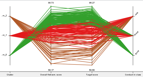 |
| Parallel plot of Conduct against target score |
The clustering model tells us that in general, students with high ‘Target scores’ generally performed well for all of their individual subjects, ‘Overall 1st sem. score’ and ‘Entrance test’ and vice versa.
Students in cluster 0 generally have the highest ‘Target score’ of 80.99, cluster 2 have the lowest ‘Target score’ with 74.589 and cluster 1 is in the middle with 66.33. The parallel coordinate plot tells us that in general, students in cluster 0 have either ‘very-good’ or ‘good’ conduct. Cluster 1 generally has ‘good’ or ‘moderate’ conduct and cluster 2 generally has ‘moderate’ conduct. This is consistent with our findings in milestone 1 where we discovered that students with poorer conduct have poorer ‘Target scores’.
Model(students not taking science)
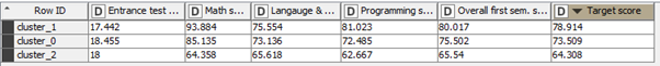 |
| Statistics of Conduct against target score |
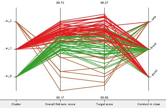 |
| Parallel plot of Conduct against target score |
Similar to ‘students taking science’, ‘students not taking science’ with high ‘Target scores’ generally performed well for all of their individual subjects, ‘Overall 1st sem. score’ and ‘Entrance test’ and vice versa.
Students in cluster 1 generally have the highest ‘Target score’ of 78.914, cluster 2 have the lowest ‘Target score’ with 73.509 and cluster 1 is in the middle with 64.308. Unlike ‘students taking science’, the parallel coordinate plot tells us that the conduct grades ‘students not taking science’ are less clearly separated. While students with ‘good’ conduct grades are generally from cluster 1 and cluster 0, conduct grades of ‘good’ and ‘moderate’ have students from all 3 clusters. However, students from cluster 2 can still be seen as having worse conduct grades than the other 2 clusters.
In conclusion, for students taking science, students with moderate conduct grades tend to have poorer ‘Target scores’ and vice versa. For students not taking science, the conduct grades of students are less clear cut, but the trend of students with poor conduct grades tend to have poorer ‘Target scores’ still holds true. ‘Target scores’ is the aggregate of all individual subjects, hence students with worse ‘Target scores’ generally have worse individual subject scores. Hence, we can deduce that those students sorted to cluster_2 will be the students in need.
4B. Modelling with Decision tree
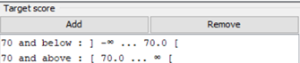
For the purposes of this analysis, the team decided that students who scored less than 70% for their target scores will be considered at risk. The team binned ‘Target score’ using the following settings. The reason behind this action is to group the students considered ‘At-risk’ together to better discover trends present. Below are the settings that the team used to build our model. All variables were used in the modelling of the decision tree.
| Settings | Rationale |
|---|---|
 |
‘Numeric binner node’ settings, explained above |
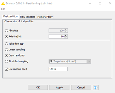 |
‘Partitioning node’ settings, the team re-used what we had learned during the course. 80% of the data is used for training and 20% is used for testing. This gives enough data for the training set to train the model while having sufficient data leftover for testing. Random seed is set to ‘12345’, making it a fixed seed. This is to ensure that partitioning of data is done in the same way every time. |
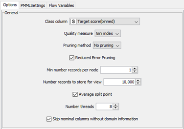 |
‘Decision tree settings.’ ‘Min number records per node’ was set to ‘1’ as the team wanted to have the maximum granularity possible for the decision tree; this will generate the most detailed tree possible. ‘Gini index’ is used to calculate the probability that a variable is classified wrongly if randomly selected. Reduced error pruning is used to cut the tree during post-processing. Every node is replaced with its most popular class if the prediction accuracy is not reduced. |
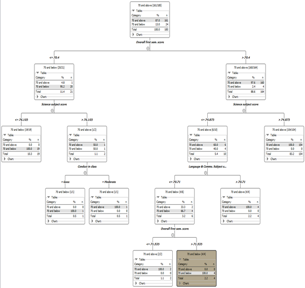
The team will first examine ‘Students taking science’
 |
|---|
| Fully expanded decision tree |
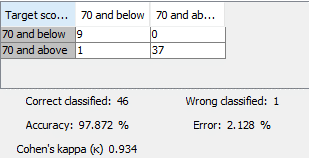 |
| Confusion matrix |
Examining the decision tree generated, the model determined that ‘Overall 1st sem score’, ‘Science subject score’, ‘Language and Comms. subject score’ and ‘Conduct in class’ are the most important variables to determine ‘Target score’.
There are 24 students the team considers ‘at-risk’. The first split in the tree occurs when ‘Overall 1st sem score’ is above or below 70.4. 20 of the 24 ‘at-risk’ students scored below 70.4 for ‘Overall 1st sem score’. The second split occurs when ‘Science subject score’ is above or below 76.105. 19 of the 20 students scored below 76.105 with only 1 scoring above that value. This is where this branch of the decision tree terminates.
For the 4 of the 24 ‘at-risk’ students, the second split occurs when ‘Science subject score’ is above or below 74.875. All 4 of the ‘at-risk’ students scored below 74.875 for ‘Science subject score’. This led to the third split when ‘Language and Comms. subject score’ is above or below 70.71. All 4 students scored more than or equal 70.71. This led to the final split when ‘Overall 1st sem score’ is above or below 71.535. All 4 students scored less than 71.535.
This shows us that in general, most ‘at-risk’ students taking science scored less than 71.535 for ‘Overall 1st sem score’, less than 74.875 for ‘Science subject score’.
Looking at the confusion matrix, the model is highly accurate at 97.872% with only one false positive. Where ‘70 and below’ is considered positive and ‘70 and above’ is considered negative.
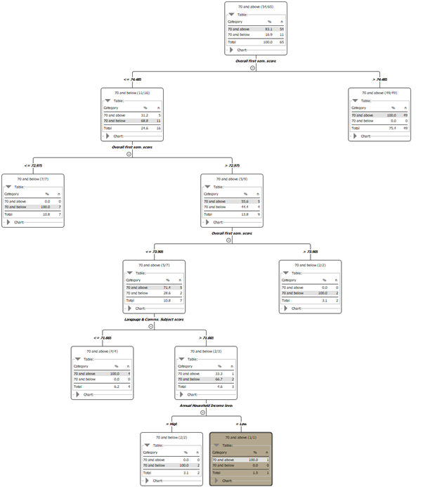
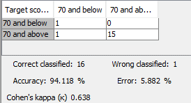
The team will first examine ‘Students not taking science’
 |
|---|
| Fully expanded decision tree |
 |
| Confusion matrix |
The model determined ‘Overall 1st sem score’, and ’Language and Comms. subject score’ are the most important variables to determine ‘Target score’ for students not taking science.
There are 11 students the team considers ‘at-risk’. The first split in the tree occurs when ‘Overall 1st sem score’ is above or below 74.485. All 11 ‘at-risk’ students scored below 74.485 for ‘Overall 1st sem score’. The second split occurs when ‘Overall 1st sem score’ is above or below 72.975. 7 of the 11 students scored below 72.975 with only 4 scoring above that value. This leads to the third split when ‘Overall 1st sem score’ is above or below 73.905. 2 of the 4 ‘at-risk’ scored less than 73.905. The fourth split occurs when ’Language and Comms. subject score’ is above or below 71.665. Both of the students scored less than 71.665 for ’Language and Comms. subject score’ and both are from high income households.
This tells us that in general, ‘at-risk’ students who did not take science scored less than 74.485 for ‘Overall 1st sem score’.
The confusion matrix tells us that the model is highly accurate at 94.118% with only one false positive. Where ‘70 and below’ is considered positive and ‘70 and above’ is considered negative.
From the decision tree model, it appears that the most important variables that predict ‘target score’ are ‘Overall 1st sem score’ and ‘Science subject score’(if applicable).
4C. Modelling with Linear Regression Below is the settings of the partitioning node used for linear regression
| Step number | Nodes used | Rationale |
|---|---|---|
| Relative[%] | 80% | Similar to the decision tree model, 80% of the data is used for training and 20% is used for testing. This gives enough data for the training set to train the model while having sufficient data leftover for testing |
| Draw randomly | - | Random sampling is used as we wanted an unbiased representation of the data |
| Random seed | 1234 | Random seed is set to ‘1234’, hence making it a fixed seed. This is to ensure that partitioning of data is done in the same way every time. |
For the model, all variables are used except for the following
| Variable | Rationale |
|---|---|
| Student ID | Student ID is a unique identification number given to students, similar in nature to a name. Hence no meaningful data can be extracted from the variable. |
| Overall first sem. att. | [see explanation below] |
The following table is the result of including ‘Overall first sem. att.’ in model of ‘Students not taking science’
 |
The team discovered the removal of ‘Overall first sem. att.’ would resolve the issue of all other attendance related variables having extreme coefficient values. However, the team was unable to ascertain as to why exactly that was the case. As such, for the sake of standardisation, ‘Overall first sem. att.’ will be omitted from all linear regression models.
The following are the result of the linear regression nodes
 |
 |
| students taking science | students not taking science |
The following are the output of the numeric scorer node for both groups of students before backwards elimination. It is important to note that as there are no students with disciplinary records in the model ‘Students not taking science’, the model omitted the variable despite the team including it in the settings of the ‘Linear Regression Learner’ node.
 |
 |
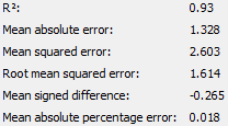
| students taking science | students not taking science |
2 linear regression models will be created. The first model, henceforth known as model 1 will investigate how individual subject scores contribute to the ‘Target score’ along with ‘Overall first sem. score’. The second model, henceforth known as model 2, will investigate how all other factors affect ‘Target score’, including interactions.
Model 1
‘Target score’ is the aggregate of all individual subject scores, as such the team wanted to investigate how each individual subject contributed to ‘Target score’. ‘Overall first sem. score’ was also separated into its own model as backward elimination done by the team resulted in only ‘Overall first sem. score’ remaining. Similarly, backward elimination done without ‘Overall first sem. score’ resulted in individual subject scores remaining. Hence the team separated these variables. Below are the results of model 1.
 |
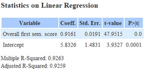 |
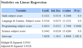
| Individual subject score for ‘Students taking science’ | ‘Overall first sem. score’ for ‘Students taking science’ |
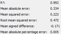
The R-Squared value of individual subjects is close to 1 and all P-values are at or close to 0 as individual subject scores contribute directly to the ‘Target score’. R-Squared and Adjusted R-Squared are both close to each other, indicating that the model does not suffer from overfitting.
The coefficient of all values tells us that the variable that contributes most to the ‘Target score’ is ‘Science subject score’ with 0.3442 followed by ‘Language & Comms. Subject score’ with 0.3316. This translates to having an average increase in ‘Target score’ of 0.3442 and 0.3316 for every 1% increase in ‘Science subject score’ and ‘Language & Comms. Subject score’ respectively.
The R-Squared and Adjusted R-Squared value of ‘Overall first sem. score’ is close to 1 and each other, indicating that the model does not suffer from overfitting. The P value of 0 also indicates that ‘Overall first sem. score’ is significant in predicting ‘Target score’.
The coefficient of ‘Overall first sem. score’ tells us that there is an average increase in ‘Target score’ of 0.9161 for every 1 point in ‘Overall first sem. score’. This implies that in general, those who did well during their 1st semester will continue to do well and vice versa.
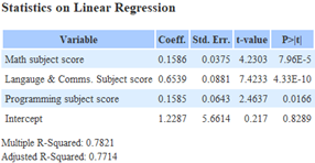 |
 |
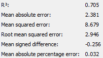
| Individual subject score for ‘Students not taking science’ | ‘Overall first sem. score’ for ‘Students not taking science’ |
All P-values are less than 0.05 as individual subject scores directly impacting ‘Target score’. R-Squared and Adjusted R-Squared is also very close to each other, indicating that the model does not suffer from overfitting. However, the R-Squared value of 0.7821, while being somewhat close to 1, tells us that individual subject scores alone may not adequately explain variation in ‘Target score’. The coefficient of all values tells us that the variable that contributes most to the ‘Target score’ is ‘Language & Comms. Subject score’ with 0.6539. This translates to having an average increase in ‘Target score’ of 0.6539 for every 1% increase in ‘Language & Comms. Subject score’.
The R-Squared and Adjusted R-Squared value of ‘Overall first sem. score’ is close to each other, indicating that the model does not suffer from overfitting. However, the R-Squared value of ‘Overall first sem. score’ is 0.7929, signifying that ‘Overall first sem. score’ may not adequately explain variation in ‘Target score’. However the P value of 0 indicates that ‘Overall first sem. score’ is significant in predicting ‘Target score’.
The coefficient of ‘Overall first sem. score’ tells us that there is an average increase in ‘Target score’ of 0.994 for every 1% increase in ‘Overall first sem. score’. This implies that in general, those who did well during their 1st semester will continue to do well and vice versa.
This finding surprised the team as we did not expect ‘Language & Comms. Subject score’ and ‘Science’ subject score’ to affect ‘Target score’ this heavily. As such we believe that students who struggle with languages would have an overall weaker ‘Target score’ and would require more assistance in their academics. However, if the student is taking science, then resources should be provisioned between science and languages as both have a similar impact on ‘Target score’. Furthermore, students who did poorly for their 1st semester should be monitored carefully as students generally perform similarly for their 1st semester and at the final stage.
Model 2
Based on the findings of Milestone 1, the team determined that ‘Entrance scores’, ’Conduct’ and ‘Disciplinary Warning’ have an effect on ‘Target score’. As such the following variables were added to account for interaction between variables
| Variable Name | Interaction |
|---|---|
| Ent*1_sem | Entrance scores x Overall 1st semester score |
| Con*1_sem | Conduct x Overall 1st semester score |
| Disc*1_sem | Disciplinary warning x Overall 1st semester score |
It is also noted that adapting ’Conduct’ and ‘Disciplinary Warning’ from string data type to number causes the R-Squared and Adjusted R-Squared value to decrease.
’Conduct’ is changed from ‘Moderate’, ‘Good’. ‘Very Good’ into ‘0’, ‘1’ and ‘2’ respectively. ‘Disciplinary Warning’ is changed from ‘N’ to ‘0’ and ‘Y’ to ‘1’.
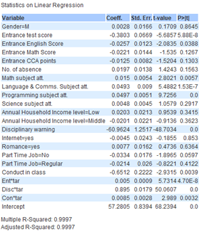 |
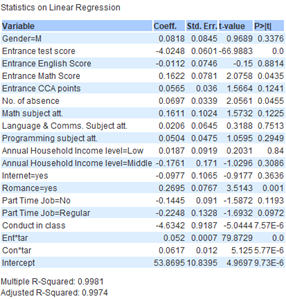 |
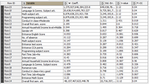
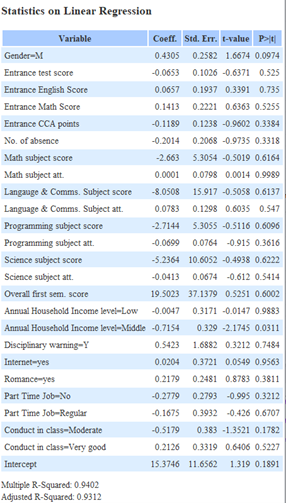
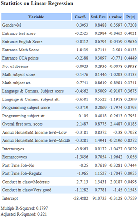
| students taking science | students not taking science |
As the linear regression node omitted ‘Disciplinary Warning’ from the model of ‘Students not taking science’, the interaction variable ‘Disc*1_sem’ will also not be included in the subsequent models of ‘Students not taking science’.
The following are the output of the numeric scorer node for both groups of students before backwards elimination.
 |
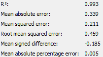 |
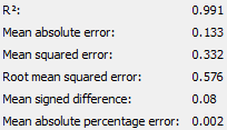
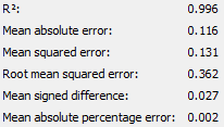
Backwards elimination will be performed on both groups of students until all variables have a P-value of less than 0.05, R-Squared is at a level the team deems satisfactory and adjusted R-Squared is close to R-Squared value.
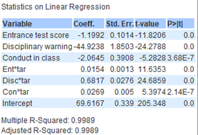
The following is the result of the backwards elimination.
 |
|
| students taking science after backwards elimination (Final model) |
students not taking science after backwards elimination (Final model) |
The following are the output of the numeric scorer node for both groups of students after backwards elimination.
 |
 |
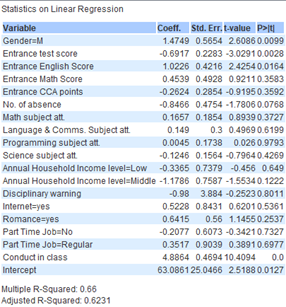
Firstly, it is important to remember that the lower the ‘Entrance test score’, the better the student did while the higher the ‘Overall 1st semester score’ the better the student did. As such it makes sense that ‘Entrance test score’ would have a negative coefficient as compared to ‘Target score’ as ‘Entrance test score’ uses a descending scale while ‘Target score’ uses an ascending scale. This is consistent with our findings in milestone 1 where we established that the better a student did for their ‘Entrance test score’ the better their ‘Target score’. From the data, on average, every 1 point increase in ‘Entrance test score’ correlates to -1.20(3sf)% decrease for ‘Target score’ for students taking science and -3.99(3sf)% decrease for those not taking science. This suggests that those with lower ‘Entrance test score’ generally did better for ‘Target score’. This also implies that students not taking science generally had slightly better entrance test scores.
As previously discovered in milestone 1, there is a relationship between ‘Target score’ and ‘Conduct in class’. In this case, every 1 point increase in ‘Conduct in class’ correlates to an average of -2.06(3sf)% for ‘Target score’ for students taking science and an average of -4.96(3sf) % for those not taking science. This is consistent with the findings of the clustering model and decision tree model implying that students with poorer conduct have lower ‘Target score’ and may require more academic help.
For students taking science, ‘Disciplinary warning’ appears to be a factor in ‘Target score’. A coefficient of -44.9(3sf) shows us that having a disciplinary record reduces the target score by -44.9(3sf) % on average. This matches our analysis in milestone 1 where students with disciplinary records generally performed worse than those without. It should also be noted that all students not taking science do not have a disciplinary record.
For students not taking science, ‘Romance = yes’ has a coefficient of 0.309(3sf), indicating that those in romantic relationships did slightly better for their target scores. This surprised the team initially, as we did not expect romance to have an impact on ‘Target score’. However after referencing our report in milestone 1, the team discovered that students not taking science in a romantic relationship did slightly better than those not in relationships, barring outliers. Here is the box plot for reference.
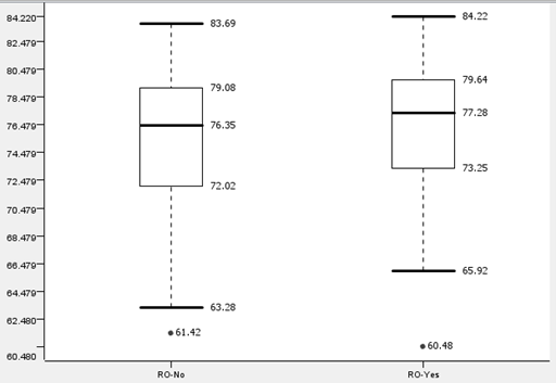
However, the team thinks that this result is an edge case for this particular cohort. Firstly, students taking science do not show this trend. Secondly, Quartile 1, Quartile 3, median and interquartile range of students with and without romantic relationships are very close to each other. Hence, the team does not think it is necessary to include ‘Romance’ as a variable for predicting target scores of students not taking science in the future.
Regarding interaction variables. Despite having relatively low coefficient, it significantly increased the R-Squared value for both groups significantly. From 0.660 to 0.9997 for students taking science and 0.4705 to 0.9981 for students not taking science prior to elimination. Included below is the model 2 without interaction variables for reference
 |
|
| students taking science without interaction variables | students not taking sciencewithout interaction variables |
As such, due to the sharp increase in R-Squared value, coupled with their P values being close to or at 0, the team concludes that ‘Target score’ interacts with ‘Entrance test scores’ , ‘Conduct in class’ and ‘Disciplinary warning’. However, the extent of their interaction and impact on ‘Target score’ is unclear as the team does not have a subject matter expert on education to consult.
The team would also like to compare the difference in R-Squared value before and after backwards elimination. For both groups, the team speculates that one or more of the variables eliminated during backwards elimination contributes to R-Squared value, despite having a P value higher than 0.05. However, the R-Squared value is still very close to 1, indicating that the variables remaining after backwards elimination explain the variation in response. The adjusted R-Squared is also very close to the R-Square value showing that neither model suffers from overfitting. Lastly, all numeric scorers are very close to 1 indicating that the models generated are very accurate in predicting ‘Target score’.
In conclusion, the linear regression model shows us that ‘Language & Comms. Subject score and ‘Science subject score’ are most likely academic predictors for ‘Target score’. ‘Overall 1st semester score’ also has a slight impact on ‘Target score’ that should not be overlooked. While ‘Entrance test scores’, ‘Conduct in class’ and ‘Disciplinary warning’(if applicable) are other possible academic predictors for ‘Target score’. As, we recommend that students who are faltering in the above fields be monitored closely and be placed into academic intervention programmes if necessary.
5. Conclusion and Evaluation
The team draws the following conclusions from trends seen from all 3 modelling techniques.
- For academic predictors, ‘Overall 1st semester score’, ‘Science subject score’ (if applicable) and ‘Language & Comms subject score’ contribute the most ‘Target Score’. ‘Entrance test score’ also has an impact.
- For non-academic predictors, ‘Conduct in class’ and ‘Disciplinary warning’ contribute the most to ‘Target score’.
Thus, our group’s main prediction model will be the linear regression and supported by the 3 other data mining techniques to help identify and intervene future ‘at risk-students’ before their final score. The team recommends the following steps be taken to aid ‘at-risk students’, which the team defines as students who scored 70 and below for ‘Target scores.
| Action | Rationale |
|---|---|
| Monitor all students with entrance scores of 18 and above | The clustering model tells us that students considered ‘at-risk’ generally scored 18 or more for their entrance test scores. |
| Monitor students who are struggling with science (if applicable) and Languages initially | Linear regression and decision tree models tell us that science (if applicable) and languages contribute the most to ‘Target score’. |
| The team recommends monitoring as some students may have difficulty adjusting to a new academic environment and struggle initially. | Linear regression and decision tree models tell us that science (if applicable) and languages contribute the most to ‘Target score’. The team recommends monitoring as some students may have difficulty adjusting to a new academic environment and struggle initially. |
| Place students who scored less than 75 for overall 1st semester into intervention programmes after 1st semester | Clustering, decision tree and linear regression model all indicate that overall 1st semester score is a key predictor for ‘Target score’. The decision tree model shows us that all students the team considers ‘at-risk’ scored 75 or less for overall 1st semester score |
| Place students who scored less than 70 for language into intervention programmes | The decision tree model shows us that all students the team considers ‘at-risk’ scored less than 70 for ‘Language & Comms. subject core’ |
| Place students who scored less than 75 for science into intervention programmes | The decision tree model shows us that all students the team considers ‘at-risk’ scored less than 75 for ‘Science subject core’ |
| Place student into disciplinary warnings into intervention programmes | The linear regression model shows us that students with disciplinary warnings generally have lower ‘Target score’ |
| Place students with conduct of ‘moderate’ into intervention programmes | Clustering and regression model shows us that students who have conduct of ‘moderate’ have lower ‘Target scores’ |